Introduction
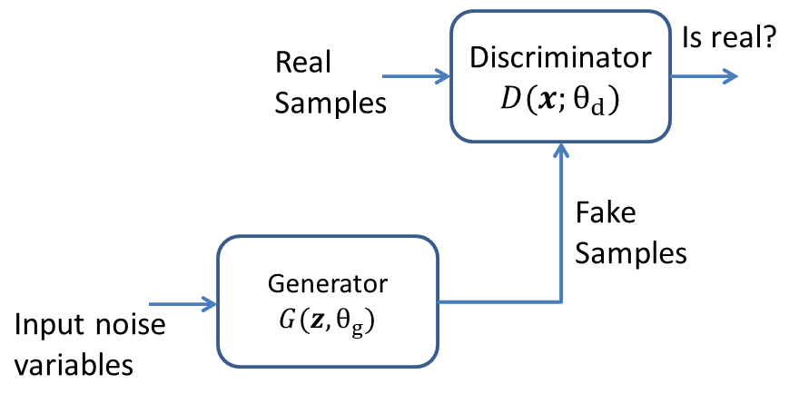
In order to generate the new samples of a distribution, it is necessary to know the data distribution $(p_{data})$. In generative adversarial networks (GANs), $p_{data}$ is approximated through generative distribution $p_g$. The GANs consists of two components, a generator $(G)$ and a discriminator $(D)$, each with learnable parameters $\theta_g$ and $\theta_d$, respectively. Also, both $G$ and $D$ are differentiable functions. We define a prior $p_\textbf{z}(\textbf{z})$, and a sample $\textbf{z}$ from this prior is mapped to data space as $G(\textbf{z};\theta_g)$. The job of discriminator is to output the probability of input sample being true $(belonging\ to\ p_{data})$ rather than generated with $G(\textbf{z};\theta_g)$ $(belonging\ to\ $(p_g)$)$. Generatorand discriminator are trained such that at convergence $p_g=p_{data}$. To quote from the original article, The generative model can be thought of as analogous to a team of counterfeiters, trying to produce fake currency and use it without detection, while the discriminative model is analogous to the police, trying to detect the counterfeit currency. Competition in this game drives both teams to improve their methods until the counterfeits are indistiguishable from the genuine articles.
Minimax Game
The role predict the probability of input sample being real. So, the $D(\cdot)$ should be $1$ if input sample is real, and zero if input sample is fake. Hence, $D(\textbf{x})$ should be one, while $D(G(\textbf{z}))$ should be zero. Hence, $D$ should minimize the following loss function: \begin{equation} \min_{D}V(D)=-E_{\textbf{x} \sim p_{data}(\textbf{x})}\left[logD(\textbf{x})\right]-E_{\textbf{z} \sim p_{\textbf{z}}(\textbf{z})}\left[log(1-D(G(\textbf{z})))\right] \end{equation} It is similar to binary cross-entropy loss. The first term will approach zero as $D(\textbf{x})$ will approach one. Similarly, second term will approach zeros when $D(G(\textbf{z}))$ will approach zero. This is precisely the motive of the discriminator. $(1)$ can be written as: \begin{equation} \max_{D}V(D)=E_{\textbf{x} \sim p_{data}(\textbf{x})}\left[logD(\textbf{x})\right]+E_{\textbf{z} \sim p_{\textbf{z}}(\textbf{z})}\left[log(1-D(G(\textbf{z})))\right] \end{equation}
As the aim of the generator is to fool the discriminator, it wants $D(G(\textbf{z}))$ to be one. Hence, $G$ want to maximize: \begin{equation} \max_{G}V(G)=-E_{\textbf{z} \sim p_{\textbf{z}}(\textbf{z})}\left[log(1-D(G(\textbf{z})))\right] \end{equation} It will be miximized when $D(G(\textbf{z}))$ is one, which is motive of the generator. (3) could be written as: \begin{equation} \min_{G}V(G)=E_{\textbf{z} \sim p_{\textbf{z}}(\textbf{z})}\left[log(1-D(G(\textbf{z})))\right] \end{equation} Combining $(2)$ and $(3)$, we get the overall objective function as: \begin{equation} \min_G \max_{D}V(D,G)=E_{\textbf{x} \sim p_{data}(\textbf{x})}\left[logD(\textbf{x})\right]+E_{\textbf{z} \sim p_{\textbf{z}}(\textbf{z})}\left[log(1-D(G(\textbf{z})))\right] \end{equation} Hence, the generator and discriminator will play a minmax game. At convergence, $D(\cdot)$ will be $0.5$, and it won’t be able to distinguish between real and fake samples.
Optimal Discriminator
For a given $G$, the $D$ is trained to maximize $V(G,D)$. \begin{equation} V(G,D)=E_{\textbf{x} \sim p_{data}(\textbf{x})}\left[logD(\textbf{x})\right]+E_{\textbf{z} \sim p_{\textbf{z}}(\textbf{z})}\left[log(1-D(G(\textbf{z})))\right] \end{equation} \begin{equation} V(G,D)=\int_x p_{data}(\textbf{x}) \left[logD(\textbf{x})\right]dx+\int_z p_z(z)\left[log(1-D(G(\textbf{z})))\right]dz \end{equation} The aim of $G$ is to produce the samples same as $\textbf{x}$ i.e. $G(\textbf{z})=\textbf{x}$ or $\textbf{z}=G^{-1}(x)$. Substituting this in $(7)$ gives: \begin{equation} V(G,D)=\int_x p_{data}(\textbf{x}) \left[logD(\textbf{x})\right]dx+\int_x p_z(G^{-1}(x))\left[log(1-D(\textbf{x}))\right]dG^{-1}(x) \end{equation} \begin{equation} V(G,D)=\int_x p_{data}(\textbf{x}) \left[logD(\textbf{x})\right]dx+\int_x p_z(G^{-1}(x))\frac{dG^{-1}(x)}{dx}\left[log(1-D(\textbf{x}))\right]dx \end{equation} \begin{equation} V(G,D)=\int_x p_{data}(\textbf{x}) \left[logD(\textbf{x})\right]dx+\int_x p_g(\textbf{x})\left[log(1-D(\textbf{x}))\right]dx \end{equation} As the $G$ is fixed, the optimal discriminator $(D^*_G(\textbf{x}))$ is obtained by maximizing the argument in $(10)$. Hence, \begin{equation} \frac{d}{dD(\textbf{x})}p_{data}(\textbf{x}) \left[logD(\textbf{x})\right]+p_g(\textbf{x})\left[log(1-D(\textbf{x}))\right]=0 \end{equation} \begin{equation} \frac{p_{data}(\textbf{x})}{D(\textbf{x})}-\frac{p_g(\textbf{x})}{1-D(\textbf{x})}=0 \end{equation} Hence, \begin{equation} D^*_G(\textbf{x})=\frac{p_{data}(\textbf{x})}{p_{data}(\textbf{x})+p_g(\textbf{x})} \end{equation}
Optimal Generator
Substituting, $(13)$ in $(10)$, we get: \begin{equation} C(G)=\int_x p_{data}(\textbf{x}) \left[log\frac{p_{data}(\textbf{x})}{p_{data}(\textbf{x})+p_g(\textbf{x})}\right]dx+\int_x p_g(\textbf{x})\left[log\frac{p_{g}(\textbf{x})}{p_{data}(\textbf{x})+p_g(\textbf{x})}\right]dx \end{equation} \begin{equation} C(G)=\int_x p_{data}(\textbf{x}) \left[log\frac{p_{data}(\textbf{x})}{\left(p_{data}(\textbf{x})+p_g(\textbf{x})\right)/2 \times 2}\right]dx+\int_x p_g(\textbf{x})\left[log\frac{p_{g}(\textbf{x})}{\left(p_{data}(\textbf{x})+p_g(\textbf{x})\right)/2 \times 2}\right]dx \end{equation} \begin{equation} C(G)=\int_x p_{data}(\textbf{x}) \left[log\frac{p_{data}(\textbf{x})}{\left(p_{data}(\textbf{x})+p_g(\textbf{x})\right)/2}-log2\right]dx+\int_x p_g(\textbf{x})\left[log\frac{p_{g}(\textbf{x})}{\left(p_{data}(\textbf{x})+p_g(\textbf{x})\right)/2}-log 2\right]dx \end{equation} \begin{equation} C(G)=\int_x p_{data}(\textbf{x}) \left[log\frac{p_{data}(\textbf{x})}{\left(p_{data}(\textbf{x})+p_g(\textbf{x})\right)/2}\right]-log2\int_x\left[p_{data}(\textbf{x})\right]dx+\int_x p_g(\textbf{x})\left[log\frac{p_{g}(\textbf{x})}{\left(p_{data}(\textbf{x})+p_g(\textbf{x})\right)/2}\right]-log 2\left[\int_x p_g(\textbf{x})\right]dx \end{equation} \begin{equation} C(G)=KL\left(p_{data}(\textbf{x})||\frac{p_{data}(\textbf{x})}{p_{data}(\textbf{x})+p_g(\textbf{x})}\right)-log2+KL\left(p_{g}(\textbf{x})||\frac{p_{data}(\textbf{x})}{p_{data}(\textbf{x})+p_g(\textbf{x})}\right)-log2, \end{equation} where first and third term is using $KL(p(x)||q(x))=\int_x p(x)log \frac{p(x)}{q(x)}dx$, and second and fourth is using $\int_x p(x)dx=1$.
\begin{equation} C(G)=2JSD\left(p_{data}(\textbf{x})||p_{g}(\textbf{x})\right)-2log2, \end{equation} JSD is Jensen–Shannon divergence and is defined as: \begin{equation} JSD(A||B)=\frac{1}{2}\left[KL\left(A||\frac{A+B}{2}\right)+KL\left(B||\frac{A+B}{2}\right)\right] \end{equation} $(19)$ can be rewritten as: \begin{equation} C(G)=2JSD\left(p_{data}(\textbf{x})||p_{g}(\textbf{x})\right)-log4, \end{equation} The role of generator is to minimize $(21)$. As $JSD\geq 0$, the minimum of $(21)$ when $JSD\left(p_{data}(\textbf{x})||p_{g}(\textbf{x})\right)=0$. This is possible when $p_{g}(\textbf{x})=p_{data}(\textbf{x})$. Hence, optimal generator is one that models the data generating process, and for that generator $C^*(G)=-log4$.
Training of GANs
Training of the GANs take place in two phases; first train the discriminator, and second train the generator. Also, from $(5)$, the aim of the generator is to minimize $E_{\textbf{z} \sim p_{\textbf{z}}(\textbf{z})}\left[log(1-D(G(\textbf{z})))\right]$. However, in the early training process, discriminator is easily able to detect the fake samples. Due to which this term won’t provide sufficient gradients. Instead the loss function is modified to maximize $E_{\textbf{z} \sim p_{\textbf{z}}(\textbf{z})}\left[log(D(G(\textbf{z})))\right]$. The training process of the GANs is as follows:
-
Define real labels as 1 and fake labels as 0
-
For a given generator, train the discriminator. Please note generator’s weights should not be updated during this step.
a. Take a batch of real samples. Using the real labels, calculate the loss $logD(\textbf{x})$ and update the parameters.
b. From the given generator, generate the fake samples and calculate the loss $log(1-D(G(\textbf{z})))$ using the fake labels. Again, update the parameters of the discriminator. However, parameters of the generators should not be updated.
-
Train the generator.
a. As mentioned, we want to maximize $log(D(G(\textbf{z})))$. From 2.b above, we use the fake samples generated by $G$ and again calculate the loss $log(D(G(\textbf{z})))$, however, with real labels. Again, parameters of the discriminator should not be update during this step.