Introduction
The conventional autoencoder is used for reconstructing the input sample. It uses an encoder that projects the data into a low-dimensional space or latent space. A decoder then projects this low-dimensional data back to the original dimension. This set-up is trained in an end-to-end manner to bring reconstructed samples as close to original samples. While just reconstructing the original samples may seem futile, autoencoders can be used for dimensionality reduction.
Another interesting question is: can autoencoders be used to generate the new samples? For example, once the training is completed, can a random vector be passed to the decoder to reconstruct some new sample that is not present in the training data? The answer most of the time is NO. If the random vector passed to the decoder does not belongs to the embedding learn through the training data, then the decoder will output some random noise. This is because there is no constrain on the latent space distribution. Hence, any random distribution will be learned as long as reconstruction loss is minimized. The new random vector passed to the decoder may not belong to this learned distribution, and hence the output will be random. The immediate solution is to put some constraints on the latent space distribution.
\begin{equation}
L=||x-\hat{x}||^2+D_{KL}(q(z|x)||p(z)),
\end{equation}
where, the $D_{KL}$ $(KL\ divergence)$ quantify the difference between the two distributions. As can be seen from this loss function, we are still minimizing the reconstruction loss, and $D_{KL}$ is acting as a regularization so that latent space distribution $(p(z|X))$ is bought close to some predefined distribution $(q(z))$. Once the training is completed, we can sample from the $q(z)$ to generate the new samples.
This was a highly over simplified explanation of the variational autoencoders (VAEs). We will now discuss the theory of the VAEs along with the implementation aspects.
Method
Let us assume observed data $\textbf{X}=\{\textbf{x}^i\}_{i=1}^{N}$, and unobserved continuous random variable $\textbf{z}$. The $\textbf{X}$ are generated through some random process involving $\textbf{z}$ such that $\textbf{z}$ is sampled from a prior distribution $p_{\theta}(\textbf{z})$, and then $\textbf{x}^i$ is generated using the likelihood $p_{\theta}(\textbf{x}|\textbf{z})$.
From the perspective of the coding theory, $\textbf{z}$ (unobserved variables) can be interpreted as code or latent variables. For such tasks, given the observed $\textbf{x}$, and unobserved $\textbf{z}$, we have to approximate the true posterior $p_{\theta}(\textbf{z}|\textbf{x})$. A direct approach to estimate this would be: \begin{equation} p_{\theta}(\textbf{z}|\textbf{x})=\frac{p_{\theta}(\textbf{x}|\textbf{z})p_{\theta}(\textbf{z})}{p_{\theta}(\textbf{x})} \end{equation} Also, \begin{equation} p_{\theta}(\textbf{x})=\int p_{\theta}(\textbf{x,z})d\textbf{z} \end{equation} \begin{equation} p_{\theta}(\textbf{x})=\int p_{\theta}(\textbf{x}|\textbf{z})p_{\theta}(\textbf{z})d\textbf{z} \end{equation} If we don’t make any simplifying assumptions, it can be the case where $p_{\theta}(\textbf{x})$ and hence, $p_{\theta}(\textbf{z}|\textbf{x})$ are intractable. For example, $\textbf{z}$ could be very high dimensional which will make the integrals intractable.
A solution to this problem is approximate intractable $p_{\theta}(\textbf{z}|\textbf{x})$ with $q_{\phi}(\textbf{z}|\textbf{x})$. The $q_{\phi}(\textbf{z}|\textbf{x})$ is known as recognition model. Given $\textbf{x}$, recognition model produces a distribution over $\textbf{z}$ which could have generated $\textbf{x}$. Hence, for this application it is also refered to as probabilistic encoder. Similarly, $p_{\theta}(\textbf{x}|\textbf{z})$ is a probabilistic decoder, since for a given $\textbf{z}$, it produces a distribution over $\textbf{x}$.
Given this set-up, the task is to minimize the KL divergence between $p_{\theta}(\textbf{z}|\textbf{x})$ and $q_{\phi}(\textbf{z}|\textbf{x})$ as we are approximating former with the later. The KL divergence between two distributions $p(x)$ and $q(x)$ is given as \begin{equation} D_{KL}(p(\textbf{x})||q(\textbf{x}))=\sum_\textbf{x}{p(\textbf{x})log \left(\frac{p(\textbf{x})}{q(\textbf{x})}\right)} \end{equation} \begin{equation} D_{KL}(p(\textbf{x})||q(\textbf{x}))=E_{\textbf{x}\sim p(\textbf{x})}\left[log \left(\frac{p(\textbf{x})}{q(\textbf{x})}\right)\right] \end{equation} Using the above relation, we can write \begin{equation} D_{KL}\left(q_{\phi}(\textbf{z}|\textbf{x})||p_{\theta}(\textbf{z}|\textbf{x})\right)=E_{\textbf{z}\sim q_{\phi}(\textbf{z}|\textbf{x})}\left[ log \left(\frac{q_{\phi}(\textbf{z}|\textbf{x})}{p_{\theta}(\textbf{z}|\textbf{x})}\right)\right] \end{equation} \begin{equation} D_{KL}\left(q_{\phi}(\textbf{z}|\textbf{x})||p_{\theta}(\textbf{z}|\textbf{x})\right)=E_{\textbf{z}\sim q_{\phi}(\textbf{z}|\textbf{x})}\left[ log\left( {q_{\phi}(\textbf{z}|\textbf{x})}\right)-log\left({p_{\theta}(\textbf{z}|\textbf{x})}\right)\right] \end{equation} \begin{equation} D_{KL}\left(q_{\phi}(\textbf{z}|\textbf{x})||p_{\theta}(\textbf{z}|\textbf{x})\right)=E_{\textbf{z}\sim q_{\phi}(\textbf{z}|\textbf{x})}\left[ log\left( {q_{\phi}(\textbf{z}|\textbf{x})}\right)\right]-E_{\textbf{z}\sim q_{\phi}(\textbf{z}|\textbf{x})}\left[log\left({p_{\theta}(\textbf{z}|\textbf{x})}\right)\right] \end{equation} Let’s take the second term and rewrite it in terms of the likelihood: \begin{equation} E_{\textbf{z}\sim q_{\phi}(\textbf{z}|\textbf{x})}\left[log\left({p_{\theta}(\textbf{z}|\textbf{x})}\right)\right]=E_{\textbf{z}\sim q_{\phi}(\textbf{z}|\textbf{x})}\left[log\left(\frac{p_{\theta}(\textbf{x}|\textbf{z})p_{\theta}(\textbf{z})}{p_{\theta}(\textbf{x})}\right)\right] \end{equation} \begin{equation} E_{\textbf{z}\sim q_{\phi}(\textbf{z}|\textbf{x})}\left[log\left({p_{\theta}(\textbf{z}|\textbf{x})}\right)\right]=E_{\textbf{z}\sim q_{\phi}(\textbf{z}|\textbf{x})}\left[log\left(p_{\theta}(\textbf{x}|\textbf{z})\right)+log(p_{\theta}(\textbf{z}))-log({p_{\theta}(\textbf{x}))}\right] \end{equation} $p_{\theta}(\textbf{x})$ can be moved out of the expectation. \begin{equation} E_{\textbf{z}\sim q_{\phi}(\textbf{z}|\textbf{x})}\left[log\left({p_{\theta}(\textbf{z}|\textbf{x})}\right)\right]=E_{\textbf{z}\sim q_{\phi}(\textbf{z}|\textbf{x})}\left[log\left(p_{\theta}(\textbf{x}|\textbf{z})\right)+log(p_{\theta}(\textbf{z}))\right]-log({p_{\theta}(\textbf{x}))} \end{equation} Substituting $(12)$ in $(9)$, we get \begin{align} D_{KL}\left(q_{\phi}(\textbf{z}|\textbf{x})||p_{\theta}(\textbf{z}|\textbf{x})\right)&=E_{\textbf{z}\sim q_{\phi}(\textbf{z}|\textbf{x})}\left[ log\left( {q_{\phi}(\textbf{z}|\textbf{x})}\right)\right]-E_{\textbf{z}\sim q_{\phi}(\textbf{z}|\textbf{x})}\left[log\left(p_{\theta}(\textbf{x}|\textbf{z})\right)+log(p_{\theta}(\textbf{z}))\right]+log({p_{\theta}(\textbf{x}))} \end{align}
$(13)$ can be rewritten as: \begin{equation} D_{KL}\left(q_{\phi}(\textbf{z}|\textbf{x})||p_{\theta}(\textbf{z}|\textbf{x})\right)-log({p_{\theta}(\textbf{x}))=E_{\textbf{z}\sim q_{\phi}(\textbf{z}|\textbf{x})}\left[ log\left( {q_{\phi}(\textbf{z}|\textbf{x})}\right)-log(p_{\theta}(\textbf{z}))\right]-E_{\textbf{z}\sim q_{\phi}(\textbf{z}|\textbf{x})}\left[log\left(p_{\theta}(\textbf{x}|\textbf{z})\right)\right]} \end{equation} \begin{equation} D_{KL}\left(q_{\phi}(\textbf{z}|\textbf{x})||p_{\theta}(\textbf{z}|\textbf{x})\right)-log({p_{\theta}(\textbf{x}))=E_{\textbf{z}\sim q_{\phi}(\textbf{z}|\textbf{x})}\left[ log\left( \frac{q_{\phi}(\textbf{z}|\textbf{x})}{log(p_{\theta}(\textbf{z}))}\right)\right]-E_{\textbf{z}\sim q_{\phi}(\textbf{z}|\textbf{x})}\left[log\left(p_{\theta}(\textbf{x}|\textbf{z})\right)\right]} \end{equation} \begin{equation} D_{KL}\left(q_{\phi}(\textbf{z}|\textbf{x})||p_{\theta}(\textbf{z}|\textbf{x})\right)-log({p_{\theta}(\textbf{x}))=-E_{\textbf{z}\sim q_{\phi}(\textbf{z}|\textbf{x})}\left[log\left(p_{\theta}(\textbf{x}|\textbf{z})\right)\right]}+D_{KL}\left( q_{\phi}(\textbf{z}|\textbf{x})||p_{\theta}(\textbf{z})\right) \end{equation}
Evidence Lower Bound (ELBO)
The negative of the left hand side of $(16)$ is known as ELBO. \begin{equation} \text{ELBO}=-D_{KL}\left(q_{\phi}(\textbf{z}|\textbf{x})||p_{\theta}(\textbf{z}|\textbf{x})\right)+log(p_{\theta}(\textbf{x})) \end{equation} \begin{equation} \text{ELBO}+D_{KL}\left(q_{\phi}(\textbf{z}|\textbf{x})||p_{\theta}(\textbf{z}|\textbf{x})\right)=log(p_{\theta}(\textbf{x})) \end{equation} The aim is to maximize the ELBO $(or\ minimizing\ -ELBO)$. As seen from $(17)$, it can be done by minimizing the KL-divergence between the $q_{\phi}(\textbf{z}|\textbf{x})$ and $p_{\theta}(\textbf{z}|\textbf{x})$, which is exactly our motive. But why the name ELBO? The $p_{\theta}(\textbf{x})$ is known as evidence. Consider $(18)$ where evidence is equal to sum of ELBO and $D_{KL}\left(q_{\phi}(\textbf{z}|\textbf{x})||p_{\theta}(\textbf{z}|\textbf{x})\right)$. As $D_{KL}\geq 0$, ELBO provides a lower bound on the evidence, and hence the name.
Minimizing the -ELBO is same as minimizing the RHS of $(16)$. Let’s consider each of these terms separately. The term $-E_{\textbf{z}\sim q_{\phi}(\textbf{z}|\textbf{x})}\left[log\left(p_{\theta}(\textbf{x}|\textbf{z})\right)\right]$ is noting but negative log-likelihood (NLL). For the task such as image reconstruction, $(p_{\theta}(\textbf{x}\|\textbf{z})$ is Gaussian, and this term equal to mean square error while for classification $(Bernoulli\ distribution)$ it is same as cross entropy. The second term is KL-divergence between $q_{\phi}(\textbf{z}|\textbf{x})$, and some prior $p_{\theta}(\textbf{z})$. We can consider this term as a regularization. So, the minimizing RHS of $(16)$ is same as minimizing NLL with some regularization.
The $p_{\theta}(\textbf{z})$ is a prior, and we have to choose it. This is also a disadvantage as a poorly chosen prior can lead to inferior performance. So the regularization term is bringing $q_{\phi}(\textbf{z}|\textbf{x})$, with which we are approximating the true posterior $p_{\theta}(\textbf{z}|\textbf{x}))$, close to some prior $p_{\theta}(\textbf{z})$. For VAEs, this prior is assumed to be Gaussian distribution. Although, some other priors can also be considered. Next, let’s find the KL-divergence between two Gaussian distributions.
KL divergence between two Gaussian Distributions
Consider a $N$ dimensional Gaussian distributions $p(x)$ with mean $\boldsymbol{\mu}_1$, and covariance matrix $\boldsymbol{\sigma}_1$. Similarly consider another distribution $q(x)$ with mean and covariance matrix $\boldsymbol{\mu}_2$, $\boldsymbol{\sigma}_2$, respectively. Then, the KL divergence between these two distributions is given as: \begin{equation} D_{KL}(p(x)||q(x))=\sum_x{p(x)log\left(\frac{p(x)}{q(x)}\right)}, \end{equation} where, \begin{equation} p(x)=\frac{1}{\sqrt{(2\pi)^N |\boldsymbol{\sigma}_1|}}exp-\left[\frac{1}{2}(\textbf{x}-\boldsymbol{\mu}_1)^T \boldsymbol{\sigma}_1^{-1}(\textbf{x}-\boldsymbol{\mu}_1)\right], \end{equation} \begin{equation} q(x)=\frac{1}{\sqrt{2\pi)^N |\boldsymbol{\sigma}_2|}}exp-\left[\frac{1}{2}(\textbf{x}-\boldsymbol{\mu}_2)^T \boldsymbol{\sigma}_2^{-1}(\textbf{x}-\boldsymbol{\mu}_2)\right], \end{equation} Substituting these in $(19)$ and solving it will lead to: \begin{equation} D_{KL}(p(x)||q(x))=\frac{1}{2}\left[log\frac{|\boldsymbol{\sigma}_2|}{|\boldsymbol{\sigma}_1|}+tr(\boldsymbol{\sigma}_2^{-1}\boldsymbol{\sigma}_1)+(\boldsymbol{\mu}_1-\boldsymbol{\mu}_2)^T\boldsymbol{\sigma}_2^{-1}(\boldsymbol{\mu}_1-\boldsymbol{\mu}_2)-N\right] \end{equation}
If $\boldsymbol{\sigma}_2=1$, and $\boldsymbol{\mu}_2=0$, i.e. $q(x)=N(0,1)$ \begin{equation} D_{KL}(p(x)||q(x))=\frac{1}{2}\left[log\frac{1}{|\boldsymbol{\sigma}_1|}+tr(\boldsymbol{\sigma}_1)+(\boldsymbol{\mu}_1)^T(\boldsymbol{\mu}_1)-N\right] \end{equation} \begin{equation} D_{KL}(p(x)||q(x))=\frac{1}{2}\left[-log{|\boldsymbol{\sigma}_1|}+tr(\boldsymbol{\sigma}_1)+\boldsymbol{\mu}_1^2-N\right] \end{equation}
As $\boldsymbol{\sigma}_1$ is a diagonal matrix. it can be implemented as vector, in which case $(24)$ can be written as:
\begin{equation}
D_{KL}(p(x)||q(x))=\frac{1}{2}\left[-log\prod_N\boldsymbol{\sigma}_1+\sum_N\boldsymbol{\sigma}_1+\sum_N\boldsymbol{\mu}_1^2-\sum_N{1}\right]
\end{equation}
\begin{equation}
D_{KL}(p(x)||q(x))=\frac{1}{2}\left[-\sum_Nlog({\boldsymbol{\sigma}_1})+\sum_N\boldsymbol{\sigma}_1+\sum_N\boldsymbol{\mu}_1^2-\sum_N{1}\right]
\end{equation}
\begin{equation}
D_{KL}(p(x)||q(x))=\frac{1}{2}\sum_N\left[-log({\boldsymbol{\sigma}_1})+\boldsymbol{\sigma}_1+\boldsymbol{\mu}_1^2-{1}\right]
\end{equation}
Using $(27)$,
\begin{equation}
D_{KL}\left( q_{\phi}(\textbf{z}|\textbf{x})||p_{\theta}(\textbf{z})\right)=\frac{1}{2}\sum_N\left[-log({\boldsymbol{\sigma}}(\textbf{x}))+\boldsymbol{\sigma}(\textbf{x})+\boldsymbol{\mu}^2(\textbf{x})-{1}\right]
\end{equation}
i.e we are assuming prior to be $N(0,1)$. Also, note that prior
doesn’t have parameters in this case. Using all these discussed concepts, the VAE can be represented as shown in figure.
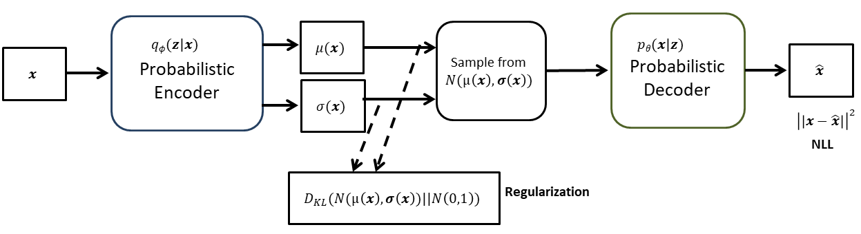
There is still one issue left to address. Is this architecture trainable through backpropagation? No, because the it involves sampling which is not a differentiable operation. The solution this problem lies in what is called ‘reparameterization trick’.
Reparameterization Trick
Given a sample from $N(\mu, \sigma)$, it can be normalized to $\mu=0$, and $\sigma=1$ as: \begin{equation} x’=\frac{x-\mu}{\sqrt{\sigma}} \end{equation} Hence, \begin{equation} x=\mu+x’\sqrt{\sigma} \end{equation} Now, instead of sampling from $N(\mu(\textbf{x}), \sigma(\textbf{x}))$, we can sample from $N(0,1)$, and then can apply $(25)$. It will be similar to sampling from $N(\mu(\textbf{x}), \sigma(\textbf{x}))$. Incorporating this, the final VAE block diagram is as:
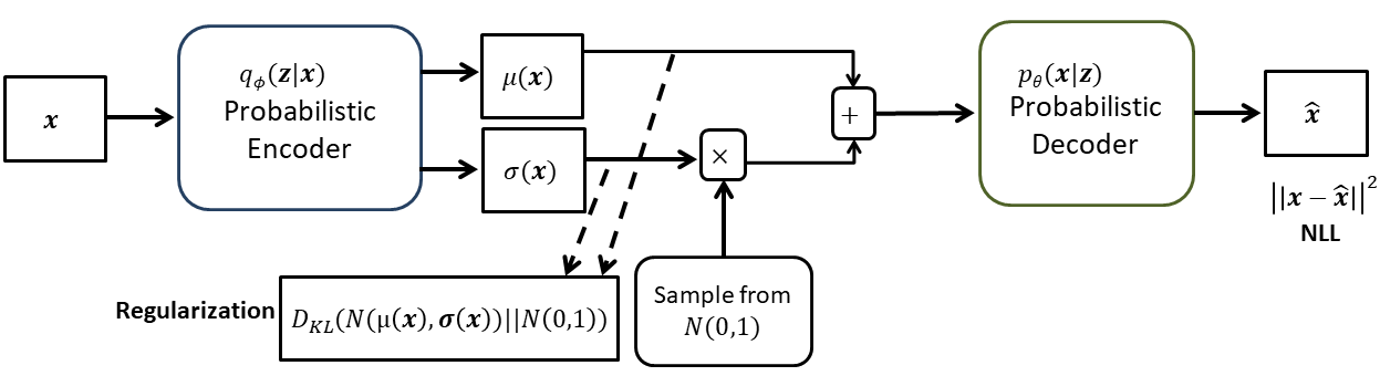
As the sampling operation has been moved out, the network can be trained with the backpropagation.
The PyTorch implementation of the VAEs can be found [here]