Introduction
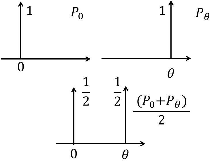
Consider two distributions $P_0$ and $P_{\theta}$ as shown in figure. $P_0$ has unit value at origin, and zero otherwise. Similarly, $P_{\theta}$ is non-zero only at $\theta$. This is an example of two parallel lines. Let’s check how different distances behaves for such a case.
1. The Total Variation (TV) distance: \
\begin{equation}
\delta(P_0, P_{\theta})=\underset{x \in X}{sup}|P_0(x)-P_{\theta}(x)|
\end{equation}
For the above above example,
\begin{equation}
\delta(P_0, P_{\theta})_{{x=0}}=|1-0|=1
\end{equation}
Similarly,
\begin{equation}
\delta(P_0, P_{\theta})_{{x=\theta}}=|0-1|=1
\end{equation}
However, if $\theta=0$,
\begin{equation}
\delta(P_0, P_{\theta})_{{x=\theta=0}}=|1-1|=0
\end{equation}
Hence,
\begin{equation}
\begin{aligned}
\delta(P_0, P_{\theta}) &= 1\ \ if\ \ \theta \neq 0
&=0\ \ if\ \ \theta = 0
\end{aligned}
\end{equation}
2. The Kullback-Leibler (KL) divergence
\begin{equation}
KL(P_0||P_{\theta})=\sum_{x \in X} P_0(x) log\frac{P_0(x)}{P_{\theta}(x)}
\end{equation}
Also, KL divergence is not symmetric, hence, $KL(P_0||P_{\theta}) \neq KL(P_{\theta}||P_0)$
\begin{equation}
\begin{aligned}
KL(P_0||P_{\theta}) &= P_0(0) log\frac{P_0(0)}{P_{\theta}(0)}+P_0(\theta) log\frac{P_0(\theta)}{P_{\theta}(\theta)}
&=1 log\frac{1}{0}+0 log\frac{0}{1}
&= +\infty
\end{aligned}
\end{equation}
If $\theta=0$
\begin{equation}
KL(P_0||P_{\theta})= P_0(0) log\frac{P_0(0)}{P_{\theta}(0)}=P_0(\theta) log\frac{P_0(\theta)}{P_{\theta}(\theta)}=1log\frac{1}{1}=0
\end{equation}
Hence,
\begin{equation}
\begin{aligned}
KL(P_0|| P_{\theta}) &= +\infty\ \ if\ \ \theta \neq 0
&=0\ \ if\ \ \theta = 0
\end{aligned}
\end{equation}
Similarly, it can be shown that:
\begin{equation}
\begin{aligned}
KL(P_{\theta}||P_0) &= +\infty\ \ if\ \ \theta \neq 0
&=0\ \ if\ \ \theta = 0
\end{aligned}
\end{equation}
3. The Jensen-Shannon (JS) divergence
The JS divergence is given as:
\begin{equation}
JS(P_0,P_{\theta})=\frac{1}{2}\left[KL\left(P_0||\frac{P_0+P_{\theta}}{2}\right)+ KL\left(P_{\theta}||\frac{P_0+P_{\theta}}{2}\right)\right]
\end{equation}
As can be seen, JS divergence is symmetric. Also, $\frac{P_0+P_{\theta}}{2}$ is shown in figure.
\begin{equation}
KL\left(P_0||\frac{P_0+P_{\theta}}{2}\right)=1log\frac{1}{1/2}+0log\frac{0}{1/2}=log2
\end{equation}
Similarly,
\begin{equation}
KL\left(P_{\theta}||\frac{P_0+P_{\theta}}{2}\right)=0log\frac{0}{1/2}+1log\frac{1}{1/2}=log2
\end{equation}
Hence,
\begin{equation}
JS(P_0,P_{\theta})=log2
\end{equation}
Also, if $\theta=0$,
\begin{equation}
JS(P_0,P_{\theta}=0
\end{equation}
Hence,
\begin{equation}
\begin{aligned}
JS(P_0,P_{\theta}) &= log2\ \ if\ \ \theta \neq 0
&=0\ \ if\ \ \theta = 0
\end{aligned}
\end{equation}
4. Wasserstein-1:
It is also known as earth-mover’s distance. This metric is also a way to measure the distance between the two distributions. Intuitively, it can be explained as follows: If we assume each distribution as unit pile of soil, then Wasserstein distance is the cost of moving one pile over another. This is equal to product of amount of earth to be moved and mean distance it has to be moved, giving it the name earth-mover’s distance.
Mathematically, it is represented as: \begin{equation} W(P_0, P_g)=\underset{\gamma \in \prod(P_0, p_g)}{inf}E_{(x,y)\sim \gamma}\left[||x-y||\right], \end{equation} where $\gamma$ denotes the transport plan, and $inf$ denotes the infimum. According to this definition, the $W(P_0, P_g)=\theta$. As compared to above metrics, only Wasserstein distance is denoting the true distance between the two distributions. Also, this distance will reduce as two distributions will come closer. This characteristic is not shown by any of the above discussed distances. They are either constant (or infinite) when two lines are not overlapping, and zero otherwise.
Although this analysis has been shown for simple case of two parallel lines, it can be extended to other distributions as well.
Wasserstein GANs
Wasserstein GANs $(WGANs)$ make use of the Wasserstein distance in the objective function. However, the infimum in $(17)$ is intractable, and hence this equation is not implemented directly. An alternative to this equation comes from Kantorovich-Rubinstein duality, according to which \begin{equation} W(P_0, P_g)=\underset{||f||_L \leq 1}{sup}E_{x\sim P_0}[f(x)]-E_{x\sim P_{\theta}}[f(x)], \end{equation} where $sup$ is supremum. Also, $f$ denote 1-Lipschitz functions. A k-Lipschitz function $(g)$ is defined as: \begin{equation} \frac{|g(x)-g(y)|}{|x-y|}\leq k. \end{equation} i.e. it has a bounded first derivative. If $||f||_L \leq 1$ is replaced with $||f||_L \leq k$ instead, we will obtain $k.W(P_0, P_g)$, which is achieved by WGANs.
Let, $D$ be discriminator parameterized by weights $w\in W$ such that $D_w(\cdot)$ represents the output of the discriminator. Also, let $G_{\theta}$ be the generator with parameters $\theta$, and $G_{\theta} (\cdot)$ represents the output of the generator. If $x$ represent the real sample, and $z$ represents the sample from the latent space, then $D_w(x)$ is the output of the discriminator for the real sample, and $G_{\theta} (z)$ is the fake sample generated by the generator. Also, $D_w(G_{\theta} (z))$ is the output of the discriminator for fake samples. Also, if $D_w$ K-Lipschitz for some $K$, we can rewrite $(18)$ as: \begin{equation} W(P_0, P_g)=\underset{||D_w||_L \leq k}{sup}E_{x\sim P_0}[D_w(x)]-E_{z\sim p(z)}[D_w(G_{\theta} (z))], \end{equation} Hence, this will yield $K$ multiplicative Wasserstein distance. It can be simplified to: \begin{equation} \max_{w \in W}E_{x\sim P_0}[D_w(x)]-E_{z\sim p(z)}[D_w(G_{\theta} (z))] \end{equation} This is the objective function for the discriminator i.e. it wants to maximize the Wasserstein distance between the two distributions. Generator on the other hand, wants to minimize this distance. Hence for generator: \begin{equation} \min_{\theta}-E_{z\sim p(z)}[D_w(G_{\theta} (z))] \end{equation} For implementation, instead of maximizing $(21)$, we minimize \begin{equation} \min_{w \in W}-E_{x\sim P_0}[D_w(x)]+E_{z\sim p(z)}[D_w(G_{\theta} (z))] \end{equation} Also note that unlike the classical GANs, the discriminator is not giving a decision if the sample is real or fake. Instead its telling the closeness of the two distributions. From this perspective, discriminator is called critic in the WGANs.
A critic $(D_w)$ that maximize $(21)$ or minimize $(23)$, can be implemented with a neural networks with weights $w$ that lie in compact space $W$. This will ensure that $D_w$ will be $K$-Lipschitz for some $K$. The space can be made compact by clamping the weights to a box i.e. $W=[-.001,.01]^l$. This is done after each gradient update. However, there are disadvantages of using this approach to enforce Lipschitz constraint. A large clipping parameter will lead to slow training of the critic, and hence critic will take longer to reach optimality. On the other hand, a smaller clipping parameter may lead to vanishing gradient problem in the case of deeper architectures or in the absence of batch normalization. After this work, spectral normalization was proposed to enforce Lipschitz constraint. Spectral normalization is very effective in stabilizing the training of the GANs.
Training of WGANs
The sample code for training the WGANs in PyTorch can be given as follows. Let generator and critic are implemented using a neural network. $z$ be noise sample given to the generator for producing the fake samples. Optim_G and optim_C be the optimizers for generator and critic, respectively. n_critic be the number of iterations for training the critic, c be clipping parameter, and total_epochs be total number of the epochs.
for epoch in range(total_epochs):
## Train the critic for n_critic
    for n in range(n_critic)
        optimizer_C.zero_grad()
        ## Take real samples
        real_samples = Variable(imgs)

        ## Take noise samples and generate fake samples
        fake_samples = generator(z).detach()
        ## Find the loss using (23)
        loss_C = -torch.mean(critic(real_samples)) + torch.mean(critic(fake_samples))
        ## Update the parameters of the critic
        loss_C.backward()
        optimizer_C.step()
        ## Constrain the parameters to a fixed box defined by c
        for parms in critic.parameters():
            params.data.clamp_(-c, c)

    ## Train generator
    optim_G.zero_grad()

    # Generate fake samples
    ## Take noise samples and generate fake samples
    fake_samples = generator(z)
    # Find the loss using (22)
    loss_G = -torch.mean(critic(fake_samples))
    ## update the generator
    loss_G.backward()
    optimizer_G.step()